
What Is VLOOKUP in Google Sheets?
A well-liked and adaptable spreadsheet tool, Google Sheets makes it simple for users to organise and analyse data. The VLOOKUP function, which enables users to search for a certain value in a table and get the comparable value from another column in the same table, is one of Google Sheets’ most significant features.
The VLOOKUP Google sheets function is very handy when dealing with big data sets, since it may swiftly search and retrieve information with only a few clicks. You must first specify the value you want to search for, the range of cells that make up the table, the column index number of the value you want to get, and whether you want an exact or approximate match before you can use the VLOOKUP function.
Let’s say, for example, that you have a table with a list of goods and their associated prices. You’re looking for “Widget A’s” price, specifically. The steps below will show you how to use the VLOOKUP function to accomplish this:.
- Select the cell where you want to display the result.
- Type the VLOOKUP function, starting with the equal sign (=VLOOKUP).
- Enter the value you want to search for, in this case “Widget A”.
- Specify the range of cells that contains the table, including the column that contains the value you want to retrieve.
- Enter the column index number of the value you want to retrieve, counting from left to right starting with the first column in the range.
- Specify whether you want an exact or approximate match, depending on your needs.
Following the completion of these steps, the VLOOKUP function will scan the table for the value “Widget A” and return the price associated with that value from the specified column.
In conclusion, the function VLOOKUP Google Sheets is a key tool for anyone who needs to work with large data sets. By mastering this feature, you can speed up your workflow and save time so that you can concentrate on what really matters—analyzing and evaluating your data to make wise decisions.
VLOOKUP Google Sheets Function
A built-in function in Google Sheets called VLOOKUP enables searching across multiple columns.
It is typed =VLOOKUP and has the following parts:
=VLOOKUP(search_key, range, index, [is_sorted])
Note: The column that contains the lookup’s data must always be on the left.
Each of the VLOOKUP formula’s parameters delivers the following:
- key: the value that the function uses to search the other column
- range: Defines the cell ranges to search for the data in.
- index: specifies the searchable column. The first column is denoted by the number 1. Between 1 and the total number of columns, the value must fall.
- is-sorted: Specifies whether or not the range is sorted through an optional argument. The value is TRUE by default if left empty. If your data is not sorted, you can also type FALSE.
Also read: How to Merge Cells in Google Sheets Learn easily Step-by-Step
Examples of VLOOKUP Google Sheets function
Due to some of its nuances, VLOOKUP can be a little challenging to use. To help you interpret how the formula works, here are a few examples.
How to use a Simple VLOOKUP google sheets
The VLOOKUP function can be used to find a cell that matches a user reference by referencing a cell in the first parameter and a range in the second.
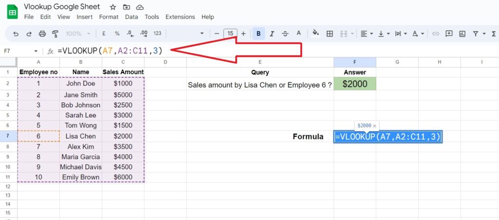
In the example that follows, we’ll pretend that we need to locate Employee 6 sales information. Although it’s simple to see the solution in a small spreadsheet, you can imagine that performing a straightforward VLOOKUP would save a tonne of time with thousands of rows of data.
- Open Google Sheets spreadsheet document.
- Select an empty cell.
- Type the function’s first part , which is =VLOOKUP(
- Enter the first argument in cell above example , with Employee No. 6, is A7. Type a comma
- Enter the next argument, to define the cell range. In the above example, the cell range is A1:C11. Type another comma.
- Enter the argument that specifies the search column. In this example, it is column 3. Press Enter.
or copy from here =VLOOKUP(A7,A2:C11,3)
Nested Function in VLOOKUP Google sheets
You can use a function within another formula in Google Sheets. This is known as nesting. In this case, we want to find the employee who made the fewest sales.
Finding that requires the use of Google Sheets MIN function. To accomplish this, we will use the MIN function within the VLOOKUP formula. Here are the steps you must take to accomplish this:

- Open Google Sheets spreadsheet document.
- Select an empty cell.
- Enter first part of the formula, =VLOOKUP(
- As the first argument, use the MIN function by typing MIN(. A nested formula does not require an equals sign.)
- Enter the range to be checked in order to find the minimum value. In the preceding example, it is A2:A11.
- Now close the bracket for MIN formula
- Enter the formula’s cell range. The range in this example is A1:C11.
- To search, enter the column index number. In the preceding example, it is 3.
- Because the data we have is not sorted, type FALSE for the last argument.
- Enter closing bracket for the formula.
- To start the search, press Enter.
Copy formula: =VLOOKUP(MIN(A2:A11),A2:C11,3,FALSE)
Continue Your Search Using Google Sheets VLOOKUP Function
The function VLOOKUP google sheets is extremely useful, but it cannot always perform the exact search you require. There are numerous other search functions in Google Sheets, and even more across the entire Google Apps suite. Continue to learn, and you’ll be a Google Apps expert in no time.